Introduction
Convertible bonds combine fixed-income cash flows with equity optionality, making their pricing both financially important and technically challenging. In practice, Monte Carlo simulation is the most widely used approach for convertible bond pricing. However, achieving stable and accurate results typically requires a large number of simulated paths and fine time discretization. This makes CPU-based Monte Carlo implementations too slow for many real-time or large-scale applications. And this motivates leveraging GPU acceleration. In this post, we focus on building a CUDA-based Monte Carlo engine for convertible bond pricing.
Rather than designing a model from scratch, we build upon an existing open-source convertible bond pricing repository convertible_bond_pricing . This model was selected because it is well-documented, its validity has been verified in the original report, and it is grounded in real-world contractual provisions and real Chinese convertible bond market data, making it a solid and realistic foundation for studying GPU acceleration.
Convertible bond pricing model based on Monte Carlo method
The core logic of this convertible bond pricing model is to operate under a risk-neutral valuation framework. We use simulated stock price paths as the basic state variable and embed the bond’s contract terms explicitly along each path. By doing this, the model captures both the equity option feature and the debt cash flow structure in the convertible bonds.
Generally, the pricing procedure includes three steps:
- Simulate stock price paths: Generate future stock price paths under the risk-neutral measure, based on the stochastic process of the underlying stock.
- Apply contract clauses: Check and apply provisions dynamically—including conversion, redemption (call), put, and reset—along every simulated path to determine the cash flows and termination events.
- Discount and Average: Discount the payoff from each path back to the valuation date, then take the average across all paths to get the theoretical bond price.
In this model, we assume the stock price follows the standard Black–Scholes–Merton risk-neutral process. Put simply, we treat the stock price movement as a Geometric Brownian Motion (GBM). Under this framework, the log-return of the stock follows a normal distribution. We set the drift equal to the risk-free rate (minus dividends, if any), and for the volatility, we keep it constant—calculated based on the real stock price data from the last 60 days. For every simulated stock price path, our model evaluates the embedded clauses by checking backward along the path. The flowchart below shows how these clauses are applied:
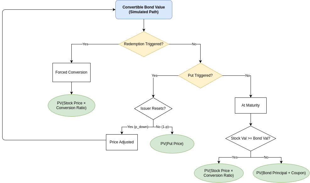
Conversion provision: Even though the conversion is legally an American-style option, we assume early conversion is not optimal because there is no dividend. Therefore, we only consider conversion at the maturity date, or when it is forced by a redemption (call) event. This assumption helps to simplify the decision logic, but it is still consistent with standard convertible bond theory.
Redemption (call) provision: When the redemption condition is satisfied on a path, we assume the issuer will call the bond. In response, the investor converts immediately, and the path terminates with the corresponding conversion payoff. This reflects the rational behavior of the investor under a forced conversion scenario.
Put and reset provisions: When a put condition is triggered, the model introduces an exogenous probability to decide whether the issuer chooses to reset the conversion price or allow the put to be exercised. The decision to reset depends on historical stock prices, which explicitly brings path dependency into the valuation. This mechanism captures the issuer’s discretion while avoiding making the game-theoretic formulation too complex. Notably, the coexistence and interaction of put and reset provisions are a distinctive feature of the Chinese convertible bond market.
CUDA Implementation and Performance Optimization
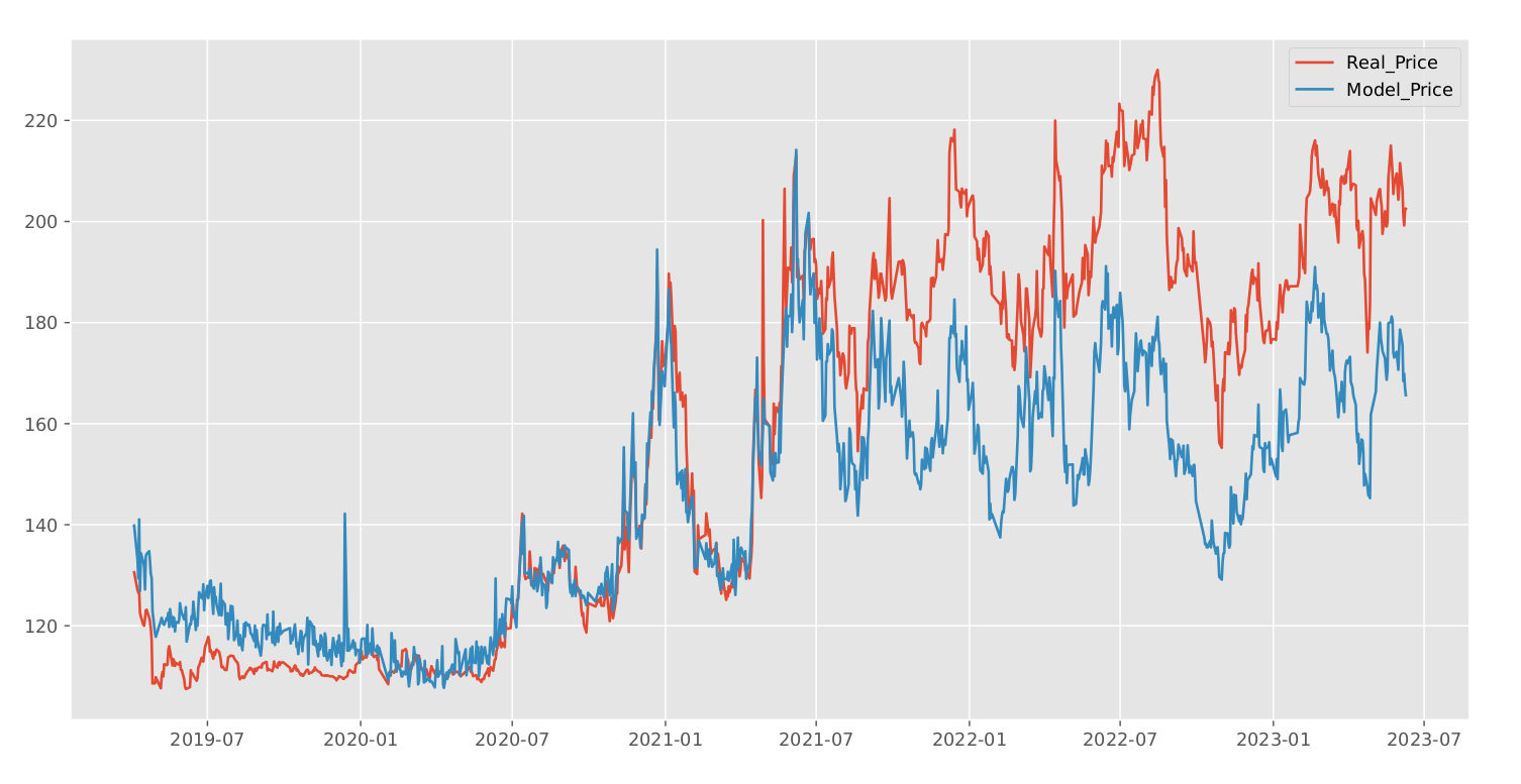
Before diving into the detailed GPU optimization journey, we first present the performance results to provide context. We develop three different CUDA kernels to execute the model, all of which achieve comparable accuracy to the CPU implementation. All experiments were conducted on a desktop equipped with an NVIDIA GeForce RTX 4060 Ti, using CUDA Toolkit 12.8. Each CUDA kernel (100,000 paths) was executed 1,000 times, with the first five runs used as warm-up. Reported timings are averages over the remaining runs. Accuracy is evaluated by computing the relative error with respect to the CPU implementation, rather than against a closed-form or “true” price. All the code is available on GitHub.
| Kernel ID | Kernel Name / Feature | Precision | Time / Speed up | Relative Error |
|---|---|---|---|---|
| 0 | CPU | FP64 | 41.304 seconds (1×) | 0% (reference) |
| 1 | Naive GPU | FP64 | 82.52 ms (500×) | 0.034% |
| 2 | Mixed Precision | FP32 / FP64 | 28.04 ms (1473×) | 0.060% |
| 3 | Mixed precision + Global memory optimization + sliding window | FP32 / FP64 | 8.01 ms (5156×) | 0.043% |
Naive GPU Baseline
We begin with a naive GPU implementation which is Kernel 1, whose primary purpose is to establish a correctness baseline rather than maximize performance.
The guiding principle at this stage is fidelity to the original Python implementation. The CUDA version closely mirrors the control flow and numerical logic of the CPU code, effectively “translating” the Python algorithm into CUDA. Each GPU thread is responsible for handling one Monte Carlo simulation path. This naive implementation ensures that the GPU and CPU implementations produce consistent results and also provides a stable reference point before introducing algorithmic refactoring and low-level optimizations, which tend to reduce code readability and complicate debugging.
Mixed-Precision Optimization
While functionally correct, the naive GPU version is far from optimal. The most obvious and impactful optimization opportunity is precision reduction.
Using full double precision (FP64) throughout the computation significantly limits performance. However, aggressively switching to single precision (FP32) can lead to excessive floating-point round-off error.
After empirical testing, we adopt a mixed-precision strategy that balances accuracy and performance resulting in Kernel 2.
FP32 is used for most intermediate computations along each Monte Carlo path. FP64 is reserved for the final accumulation step, where pathwise payoffs are summed and averaged.
This design is motivated by two considerations:
1) Error accumulation: Summation operations are particularly sensitive to precision, as rounding errors accumulate with the number of paths.
2) Output sensitivity: Operations closer to the final output have a disproportionately large impact on the final price accuracy.
This mixed-precision approach delivers substantial speedups while maintaining accuracy comparable to the CPU reference.[1] [2]
Profiling and Bottleneck Analysis with Nsight Compute
To identify the dominant performance bottlenecks, we profile the kernel using Nsight Compute, a profiling tool designed for deep-dive performance analysis of individual CUDA kernels. The full profiling report is included in the repository as well. Two major issues emerge:
Thread Divergence: Due to the complex contractual logic of convertible bonds, the kernel contains numerous conditional branches and early exits. As a result, warp-level thread divergence is significant. Unfortunately, this issue is largely inherent to the problem structure itself. The decision logic for conversion, redemption, and reset is highly path-dependent, leaving limited room for eliminating divergence without fundamentally redesigning the model.
Excessive Global Memory Access: Profiling reveals extremely high L2 (global) memory traffic, indicating excessive global memory access. The root cause lies in the original algorithm design, which stores the entire stock price history for each path. Given the large number of time steps and simulation paths, these intermediate results must reside in global device memory, leading to heavy memory bandwidth pressure.
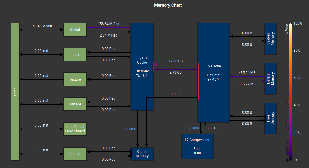
The original motivation for storing full price histories was to evaluate redemption and put conditions based on historical averages. However, closer inspection reveals that only a rolling window of past prices is required, rather than the complete history. We therefore replace full-history storage with a sliding window, which is: 1 )significantly smaller than the full time series and 2 )small enough to reside in registers or local memory instead of global memory. After applying this optimization and re-profiling the kernel (Kernel 3 ), global memory access drops dramatically(L2 to L1 transfer size: before 12.88GB, after 1.48GB), as expected. This reduction translates directly into a substantial decrease in overall runtime (from 28.04ms to 8.01 ms).

Conclusion and Future Work
We successfully implemented a CUDA-based convertible bond pricing engine that achieves significant speedups over the CPU version while maintaining comparable numerical accuracy. That said, the current implementation is far from fully optimized. Several promising directions for future work remain: Random number generation and sampling: More efficient RNG strategies or quasi–Monte Carlo methods could further reduce variance and runtime. Multi-bond parallelization: Extending the kernel to price multiple convertible bonds simultaneously would improve GPU utilization in production settings.